f-GAN: Training Generative Neural Samplers using Variational Divergence Minimization

https://arxiv.org/pdf/1606.00709.pdf

Abstract

Using an auxiliary discriminative neural network, GANs can be used to compute likelihoods or marginalizations. Since GA approach is one case of variational divergence estimation approach, any f-divergence can be used.

1. Introduction

Probabilistic generative models of Q are generally interested in:

• Sampling

  Produce a sample from Q

• Estimation

  From iid samples ${x_1, x_2, \dots, x_n}$ from unknown distribution P, find Q

• Point-wise likelihood evaluation

  evaluation of $Q(x)$ of a given sample x

GANs do exact sampling and approximate estimation. Since it needs one forward pass is needed to generate a sample, sampling is easy in GANs. It estimates a neural sampler by approximate minimization of the symmetric Jenson-shannon divergence:

\[D_{JS}(P\|Q)=0.5(D_{KL}(P\|(P+Q)/2)+D_{KL}(Q\|(P+Q)/2))\]

In this paper, researchers suggests:

• Derivation of GAN training objectives for all f-divergences
• Simplifying the saddle-point optimization procedure and justification
• Experimental evidence of suitability of divergence function for estimating generative neural samplers

2. Method

2.1. The f-divergence Family

A large class of different divergences are so called f-divergence, also known as Ali-Silvey distances. With two continuous density function p and q from two distributions P and Q, f-divergence is defined as:

\[D_f(P\|Q)=\int_\mathcal{X}q(x)f\left(\frac{p(x)}{q(x)}\right)dx\]

with the generator function $f:\mathbb{R}_+\rightarrow\mathbb{R}$ which is convex, lower-semicontinuous function with $f(1)=0$.

2.2. Variational Estimation of f-divergences

Variational divergence minimization (VDM) is a method to estimate a divergence for a fixed model, and GAN is a special form of more general VDM framework.

For every convex and lower-semicontinuous function f, there is a convex conjugate function f*, also known as Fenchel conjugate, defined as

\[f^*(t)=\sup_{u\in\,dom_f}\{u t - f(u) \}\]

Which is again convex and lower-semicontinuous, and (f, f) is dual to another as f**=f. Thus, $f(u)=\sup_{t\in\,dom_{f^}}{t u - f^*(t)}$.

From Nguyen et al., variational representation of f in the definition of the f-divergence can obtain a lower bound on the divergence:

\[\begin{align*}D_f(P\|Q)&=\int_\mathcal{X}q(x)\sup_{t\in\,dom_{f^*}}\{t \frac{p(x)}{q(x)} - f^*(t)\}dx\\&\geq\sup_{T\in\mathcal{T}}\left(\int_{\mathcal{X}}p(x)T(x)dx-\int_{\mathcal{X}}q(x)f^*(T(x))dx\right)\\&=\sup_{T\in\mathcal{T}}\left(\mathbb{E}_{x\sim\,P}[T(x)]-\mathbb{E}_{x\sim\,Q}[f^*(T(x))]\right)\end{align*}\]

For an arbitrary class $\mathcal{T}$ of functions $T:\mathcal{X}\rightarrow\mathbb{R}$. The above uses the Jensen’s inequality with integration and supremum, and the fact that class of functions may contain only a subset of all possible functions.

By taking the variation of the lower bound, tight bound of

\[T^*(x)=f'\left(\frac{p(x)}{q(x)}\right)\]

can be obtained.

2.3. Variational Divergence Minimization (VDM)

Using the variational lower bound on the f-divergence, following the generative-adversarial approach and two neural networks, Q and T, generative model Q can estimate a true distribution on P. Two networks are parameterized as $Q_\theta\textrm{ and }T_\omega$. Finding a saddle-point of the following f-GAN objective function by minimize with theta and maximize with omega:

\[F(\theta, \omega)=\mathbb{E}_{x\sim\,P}[T_\omega(x)]-\mathbb{E}_{x\sim\,Q_\theta}[f^*(T_\theta(x))]\]

Expectations can be approximated from minibatch. Distribution from P uses training set without replacement, and distribution from Q uses samples from current generative model.

2.4. Representation for the Variational Function

To consider the domain of the conjugate functions, assume the variational function can be represented as $T_\omega(x)=g_f(V_\omega(x))$. Therefore, the objective function becomes:

\[F(\theta,\omega)=\mathbb{E}_{x\sim\,P}[g_f(V_\omega(x))]+\mathbb{E}_{x\sim\,Q_\theta}[-f^*(g_f(V_\omega(x)))]\]

with $V_\omega:\mathcal{X}\rightarrow\mathbb{R}$ with no range constraints for output, and $g_f:\mathbb{R}\rightarrow\,\text{dom}_{f^*}$ of output activation function specific to current f-divergence, which is chosen as monotone increasing, as large output V(x) corresponds to the belief of the variational function that the sample x comes from the data distribution P as in the GAN case. With comparison to GAN case of:

\[F(\theta,\omega)=\mathbb{E}_{x\sim\,P}[\log{D_\omega(x)}]+\mathbb{E}_{x\sim\,Q_\theta}[\log(1-D_\omega(x))]\]

is one of a case of above, with $D_\omega(x)=1/(1+e^{-V_\omega(x)})\textrm{ and }g_f(v)=-\log(1+e^{-v})$.

2.5. Example: Univariate Mixture of Gaussians

To see the properties of f-divergences, variational divergence estimation experiment was done. With a neural network with two hidden layers, the objective F was optimized with single-step gradient method, and compared the results with numeric solution.

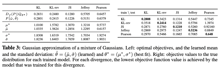
With comparison to the lower bound property, there seemed to be a good correspondence between the gap in objectives and the difference between the fitted mean and variances. The result demonstrates that if the generative model is misspecified and does not match with the real distribution, the divergence function is responsible for that.

3. Algorithms for Variational Divergence Minimization (VDM)

There is two numerical methods discussed in this paper to find saddle points of the objectives: alternating the original method from Goodfellow et al., and direct single-step optimization procedure. In variational framework, alternating gradient method is double-loop method of inner loop of tightening lower bound on the divergence, and outer loop of improving generator model.

3.1. Single-Step Gradient Method

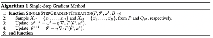
With no inner loop, the gradients with respect to omega and theta are computed in a single back-propagation.

Analysis

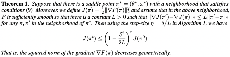
Algorithm 1 geometrically converges to a saddle point $(\theta^*, \omega^*)$ if there is a nearby neighbor around the saddle point, with F of strongly convex in $\theta$ and strongly concave in $\omega$. Therefore,

\[\nabla_\theta\,F(\theta^*,\omega^*)=0, \nabla_\omega\,F(\theta^*,\omega^*)=0, \nabla^2_\theta\,F(\theta^*,\omega^*)\succeq\delta\,I, \nabla_\theta\,F(\theta^*,\omega^*)\preceq-\delta\,I\]

and from those assumptions, next theorem proves convergence of algorithm 1.

Theorem 1

• Proof

  define $\pi^t=(\theta^t,\omega^t)$ and let

  \[\nabla\,F(\pi)=\begin{pmatrix}\nabla_\theta\,F(\theta,\omega)\\\nabla_\omega\,F(\theta,\omega)\end{pmatrix}, \tilde\nabla\,F(\pi)=\begin{pmatrix}-\nabla_\theta\,F(\theta,\omega)\\\nabla_\omega\,F(\theta,\omega)\end{pmatrix}.\]

  Then $\pi^{t+1}=\pi^t+\eta\tilde\nabla\,F(\pi^t)$.

3.2. Practical Considerations

With the finding of Goodfellw et al., more general f-GAN Algorithm can be obtained by modifing the minimizing with respect to theta part reversely:

\[\theta^{t+1}=\theta^t+\eta\nabla_\theta\mathbb{E}_{x\sim\,Q_{\theta^t}}[g_f(V_{\omega^t}(x))]\]

as in the way of maximizing $\mathbb{E}_{x\sim\,Q_\theta}[\log{D_\omega(x)]}$ instead of minimixing.

In mornitoring real and fake statistics, with the threshold with $f’(1)$, the output of the variational function can be interpretted as a true sample if the variational function $T_\omega(x)$ is larger than the threshold, or it is from the generator, if otherwise.

4. Experiments

MNIST Digits

With $z\sim\textrm{Uniform}_{100}(-1, 1)$ as a input, the generator has a two linear layers with batch normalization and ReLU activation, and a final layer with a sigmoid function. Variational functioin $V_\omega(x)$ has three linear layers with exponential linear unit in between. Adam is used for optimizer.

For evaluating, the kernel density estimation of Parzen window is used. Although there is some defacts for using KDE approach, the model for Kullback-Leibler dievergence seemed to achieve a higher holdout compare to GAN.

LSUN Natural Images

Using the same architecture as in the DCGAN work, gan objective was replaced with f-GAN objective. Neural samplers were trained with GAN, KL, suqared Hellinger divergences, and the later three showed equally realistic samples.

5. Related Work

6. Discussion

Limitation: purely generative neural samplers are unbale to provide inferences, since they xannot be conditioned on observed data.