Wasserstein Generative Adversarial Networks

https://arxiv.org/pdf/1701.07875.pdf

Abstract

Unlike traditional GAN training, with WGAN, stability of learning and meaningful learning curves can be achieved by this new algorithm.

1. Introduction

Learning probability distribution means maximizing the MLE with real data samples ${x^{(i)}}_{i=1}^D$. Finding $\theta=\arg max_{\theta\in\mathbb{R}^d}{\frac{1}{m}\sum_{i=1}^{m}\log{P_\theta(x^{(i)})}}$can solve this. On the other hand, from the real data distribution $\mathbb{P}_r$, minimizing the Kullback-Leibler divergence $KL(\mathbb{P}_r|\mathbb{P}_\theta)$ also solve this problem. For the both approach, the model density $P_\theta$ is needed. However, for low dimensional manifolds, the existence for non-negligible intersection between the model manifold and true distribution is uncertain, therefore KL distance cannot be defined. To avoid this, previous solution was to add noise term to model distribution, typically a gaussian noise with relatively high bandwidth. However, it degrades the quality of the samples and blurs the image.

Therefore, instead estimating the true density $\mathbb{P}_r$, defining a random variable Z with fixed distribution, and using a parametric function $g_\theta:\mathcal{Z}\rightarrow\mathcal{X}$ could directly generate samples following a certain distribution $\mathbb{P}_\theta$ and make it close to real distribution. In this way, unlike densities, distributions confined in low dimensional manifold can be represented, and usefully generate a sample without knowing the numerical value of the density.

Comparing with VAE, GAN offers much more flexibility with the objective function including Jenson-Shannon, f-divergences and exotic combinations, but training GAN is delicate and unstable for some reasons.

Researchers tried to measure the closeness between the model and real distributions. Therefore, they defines a distance $\rho$ to calculate the distance between two distributions.

To optimize the parameter $\theta$, defining model distribution of the model in a way that mapping of $\theta\rightarrow\mathbb{P}_\theta$ to be continuous is desirable since the continuous loss function could be achieved easily, but it defends on the way of defining distance between distributions.

2. Different Distances

$\mathcal{X}: \text{compact metric set} \\ \Sigma: \text{set of the Borel subsets of }\mathcal{X} \\ Prob(\mathcal{X}): \text{space of probability measures defined on }\mathcal{X}$

• Total Variation (TV) distance:

  \[\delta(\mathbb{P}_r,\mathbb{P}_g)=\sup_{A\in\Sigma}\vert\mathbb{P}_r(A)-\mathbb{P}_g(A)\vert\]

• Kullback-Leibler (KL) distance:

  \[KL(\mathbb{P}_r\|\mathbb{P}_g)=\int{\log\left(\frac{P_r(x)}{P_g(x)}\right)P_r(x)d\mu(x)}\]

  Assuming both distributions to be continuous.

• Jensen-Shannon (JS) divergence:

  \[JS(\mathbb{P}_r,\mathbb{P}_g)=KL(\mathbb{P}_r\|\mathbb{P}_m)+KL(\mathbb{P}_r\|\mathbb{P}_m)\]

  with $\mathbb{P}_m=(\mathbb{P}_r+\mathbb{P}_g)/2$

• Earth-Mover (EM) distance or Wasserstein-1:

  \[W(\mathbb{P}_r,\mathbb{P}_g)=\inf_{\gamma\in\prod(\mathbb{P}_r,\mathbb{P}_g)}\mathbb{E}_{(x, y)\sim\gamma}[\|x-y\|]\]

  with $\prod$ be the set of all joint distribution of $\gamma(x,y)$ of marginals respectively from real and model distribution, meaning that the cost of the optimal transform between distribution.

Under the EM distance, sequences of probability distributions can converge. The other three ones does not, as shown in below example.

As shown in the above, under the EM distance, as $\theta_t\rightarrow0$, $(\mathbb{P}{\theta_t}){t\in\mathbb{N}}\rightarrow\mathbb{P}_0$, but it is not the case with the Js, KL, or TV divergences, since the resulting loss function is not continuous.

The continuity of the Wasserstein distance is proved as below.

The relative strength of the topologies is described as below.

3. Wasserstein GAN

From the Kantorovich-Rubinstein duality,

Solving the problem becomes:

And solution f to the problem would be:

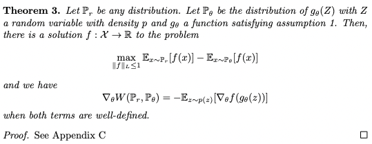
To find the function f, neural network parameterized with weights w would be the solution, and can back-propagate. However, in order to let w in a compact space, weights should be clamped in a fixed box after the gradient update. This could be problematic, since big clipping parameter needs long time to reach the limit, while small clipping size could lead to a vanishing gradient problem. But since just clipping was easy to use and showed good performance in study. Enforcing Lipschitz condition to a neural network is still left as a future investigation.

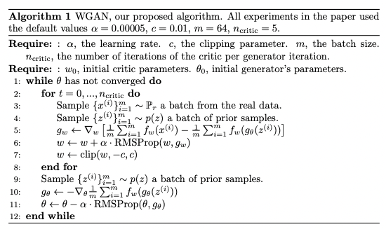
Since the normal discriminator in standard GAN quickly learn to distinguish image, it provides no reliable gradient information. However, the critic does not saturate, therefore converges to a linear function that has gradient for everywhere.

Also, due to the reason that the critic can be trained until the optimality, collapsing modes becomes harder, since mode collapse comes from the fact that the optimal generator for a fixed discriminator is a sum of deltas on the points the discriminator assigns the highest values.

4. Empirical Results

Experiments using W-GAN showed two benefits:

• meaningful loss metric correlates the generator’s convergence and sample quality
• stability of the optimization process

4.1. Experimental Procedure

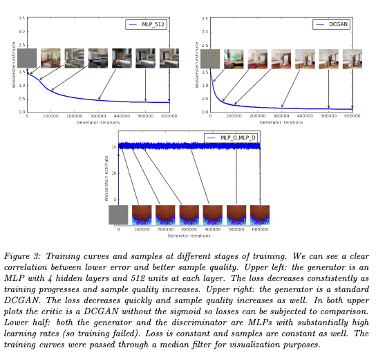
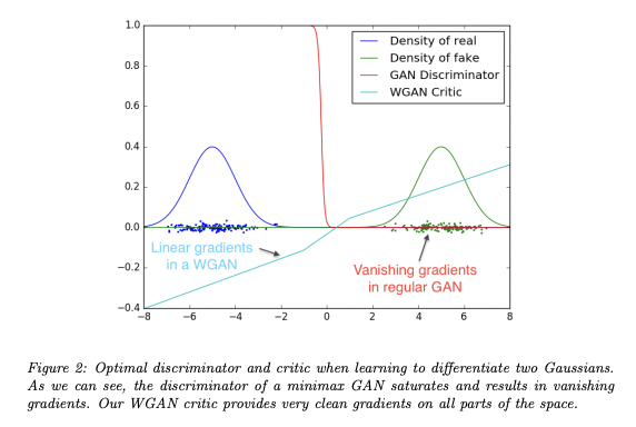
The loss constantly decreases as the training proceeds, as well as the sample quality gets increased.

4.2. Meaningful loss metric

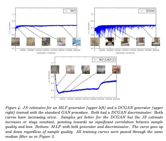
Since JS estimate usually stays constant or goes up instead of going down, the sample quality does not seem to get along with the JSD score.

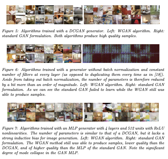
4.3. Improved stability

When the critic is trained to completion, it provides a loss to the generator that can train the neural network. Therefore, balancing generator and discriminator’s capacity properly does not play important role as before. For the experiments, there were no evidence of mode collapse for WGAN.