Attention is All You Need

https://arxiv.org/pdf/1706.03762.pdf

Abstract

Unlike previous transduction models which are based on complex recurrent or convolutional neural network including encoder and decoder, Transformer is solely based on attention mechanisms, without recurrence and convolutions. Transformer also generalizes well to other tasks.

1. Introduction

Before Transformer, long short-term memory and gated recurrent neural networks was the state of art in transduction problems such as language modeling and machine translation. There were efforts to enhance the performance of recurrent language models and encoder-decoder architectures.

Recurrent models generates a sequence of a hidden states, and this nature precludes parallelization within training examples, therefore sequential computation remains as a constraint, although there was lots of efforts with factorization tricks and conditional computation to reduce the amount of computation.

Attention mechanisms enable to modeling dependencies without regarding to distance. Transformer uses attention to draw global dependencies between input and output, without recurrence. Therefore, it allows much more parallelization.

2. Background

For ConvS2S and ByteNet, which tried to reduce sequential computation, number of operations needed increased linearly or logarithmically, thus making difficult to learn dependencies form distant positions. Unlike that, Transformer needs only a constant number of operations.

Self-attention is relating different positions of a single sequence in order to compute a representation of the sequence.

End-to-end memory networks mean models based on a recurrent attention mechanism, instead of sequence-aligned recurrence.

3. Model Architecture

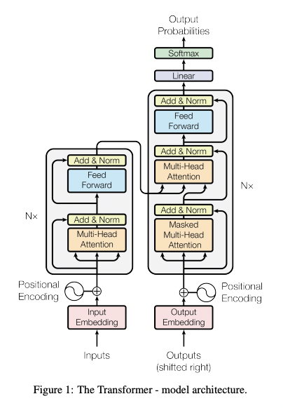
The overall architecture uses stacked self-attention and point-wise, fully connected layers for both the encoder and decoder.

3.1. Encoder and Decoder Stacks

• Encoder:

  The encoder is composed of a stack of N=6 identical layers, with each two sub-layers of multi-head self-attention mechanism and position-wise fully connected feed-forward network. A residual connection employed each layer, followed by layer normalization. Dimension of outputs is 512.

• Decoder:

  Like Encoder, the decoder is composed of N=6 identical layers. with each two sub-layer, third sub-layer of multi-head attention over the encoder stack exists in decoder. Residual connections followed by layer normalization is applied. To prevent positions from attending to subsequent positions, masking combined with fact that the output embeddings are offset by one position, ensures the predictions for position i can depend only on the known outputs at positions before i.

3.2. Attention

With vectors of the query, keys, values, and output, weight assigned to each value is computed by a compatibility function of the query with the corresponding key.

3.2.1. Scaled Dot-Product Attention

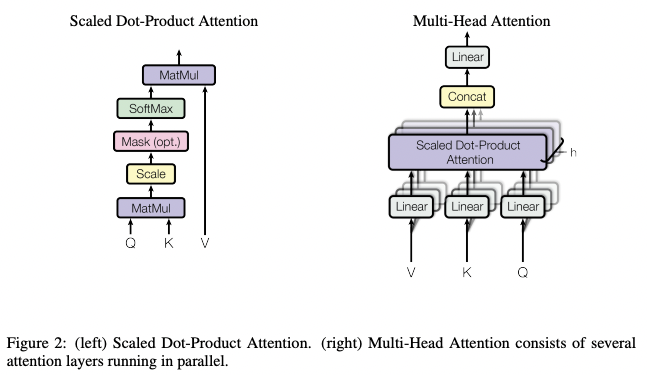
Form the left Scaled dot-product attention, attention can be calculated as:

\[\text{Attention}(Q, K, V)=\text{softmax}\left(\frac{QK^T}{\sqrt{d_k}}\right)V\]

with queries and keys of dimension $d_k$, values of dimension $d_v$. Queries and keys, values are packed into matrices Q, K and V. Unlike additive attention, which computes the compatibility function using a feed-forward network with a hidden layer, dot-product is much faster and space-efficient. Both mechanisms perform similarly in small values of $d_k$, however, since the dot product grow large in magnitude, which leads the product to the regions where the softmax function has small gradient. Therefore, the dot product was scaled by $\frac{1}{\sqrt{d_k}}$.

3.2.2. Multi-Head Attention

Linearly projecting the queries, keys, and values h times with different, learned linear projections to $d_k, d_k, d_v$ dimensions. Then performing attention in parallel, yeilds $d_v$ dimensinal output values. Concatenating and projecting again calculates final values. Multi-head attention allows the model to jointly attend to information from different representation subspaces at different positions.

\[\begin{align*}\text{MultiHead}(Q, K, V)&=\text{ConCat}(head_1, head_2, \dots, head_h)W^O,\\head_i &=\text{Attention}(QW_i^Q, KW_i^K, VW_i^V)\end{align*}\]

While $W_i^Q\in\mathbb{R}^{d_{model}\times\,d_k},W_i^K\in\mathbb{R}^{d_{model}\times\,d_k},W_i^V\in\mathbb{R}^{d_{model}\times\,d_v}\text{ and }W^O\in\mathbb{R}^{hd_v\times\,d_{model}}$.

Since the dimension of each head is reduced, total computational cost is similar to single-head attention with full dimensionality.

3.2.3 Applications of Attention in our Model

• In encoder-decoder attention layer:

  Every position in the decoder attend over all positions in the input sequence, therefore mimics the typical encoder-decoder attention mechanisms.

• Encoder:

  Each position in the encoder can attend to all positions in the previous layer of encoder.

• Decoder:

  All positions in the decoder can attend to all positions up to and including the position. Using masking, the auto-regressive property is preserved by preventing leftward information flow.

3.3. Position-wise Feed-Forward Networks

Fully connected feed-forward is consisted like below:

\[\text{FFN}(x)=\max(0, xW_1+b_1)W_2+b_2\]

And it can be treated as two convolutions with kernel size 1.

3.4. Embeddings and Softmax

Like other sequence transduction models, embeddings learned to convert input and output tokens to vector of $d_{model}$. To predict next-token probabilities, linear transformation and softmax function was used to transform the decoder output.

3.5. Positional Encoding

Without recurrence or convolution, to infer the information of sequence, positions of the tokens in the sequence should be injected. To do so, positional encodings were added at the bottoms of the encoder and decoder stacks, which has dimension of $d_{model}$.

\[\begin{align*}PE_{(pos, 2i)}&=sin(pos/10000^{2i/d_{model}})\\PE_{(pos,2i+1)}&=cos(pos/10000^{2i/d_{model}})\end{align*}\]

Using the function above, for any fixed offset k, $PE_{pos+k}$ can be represented as a linear function of $PE_{pos}$. Researchers used the sinusoidal version, since it allow model to extrapolate to sequence lengths longer than encountered during training, while the results were same.

4. Why Self-Attention

1. Total complexity per layer
2. Amount of computation that can be parallelized
3. Path length between long-range dependencies in the network

Compared to the recurrent layer requires O(n) sequential operations with sequence length n, self-attention layer is faster if n is smaller than the representation dimensionality d. For a very long sentence, self-attention should only consider a neighborhood of size r, which makes the maximum path length to O(n/r).

Convolution layer with kernel width k needs O(n/k) or O(log_k(n)) operations to connect all pairs of input and output positions. For separable convolutions, complexity considerably becomes $O(k\cdot\,n\cdot\,d+n\cdot\,d^2)$ even with k=n, which is same as self-attention layer.

5. Training

5.1. Training Data and Batching

Standard WMT 2014 English-German dataset of 4.5M sentence pairs, and WMT 2014 English-French dataset of 36M sentences were used. Batch size was approximately sequence length.

5.2. Hardware and Schedule

8 NVIDIA. P100 GPUS were used. Big models were trained for 300,000 steps with step size of 1.0 seconds.

5.3. Optimizer

Adam with $\beta_1=0.9, \beta_2=0.98\text{ and }\epsilon=10^{-9}$ was used, and the learning late was scheduled:

\[lr=d_{model}^{-0.5}\cdot\min({step\underbar{ }num}^{-0.5}, {step\underbar{ }num}\cdot\,{warmup\underbar{ }steps}^{-1.5})\]

Thus, linearly increasing learning rate for first warmup_steps, then inverse square root of the step number.

5.4. Regularization

• Residual Dropout

  Before each input and normalization of sublayers, dropout with rate of 0.1 is applied. Sums of the embeddings and the positional encodings in both encoder and decoder stacks also applied with dropout.

• Label Smoothing

  Label smoothing of $\epsilon_{ls}=0.1$ was applied. Hurts perplexity, but improves accuracy and BLEU score.

6. Results

6.1. Machine Translation

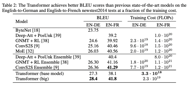
The transformer model outperformed the previous state-of-art with relatively small amount of training cost.

6.2. Model Variations

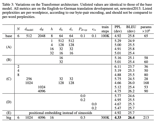
To evaluate the importance of components of Transformer, model was varied and measured in performance. Since the decrease of the attention key size $d_k$ harmed the model performance, there seemed to be an evidence of toughness of determining compatibility. Dropout helps avoiding over-fitting.

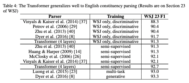
6.3. English Constituency Parsing

To test the ability to generalize of the Transformer, in semi-supervised setting, researchers trained a 4-layer transformer with $d_{model}=1024$, and it reached nearly the state-of-art with the lack of task-specific tuning, contrast to RNN sequence-to-sequence model which performed not very well.

7. Conclusion

Replacing recurrent layers in encoder-decoder architectures with multi-headed self-attention worked well for translation tasks and others, and it can be applied in many other tasks.