A Simple Framework for Contrastive Learning of Visual Representations
Abstract
By simplifying contrastive self-supervised learning algorithms, researchers show that importance of composition of data augmentations in effective predictive tasks, and learnable nonlinear transformation between the representation and the contrastive loss substantially improves the quality of the learned representations. Also, they show that contrastive learning benefits from larger batch sizes and more training steps compared to supervised learning.
1. Introduction
Most methods related to learning visual representations by unsupervised learning can be summarized by two major cases: generative or discriminative. In this case, framework for contrastive learning of visual representation is used, called SimCLR. From the systematical study of the framework, it seems that to enable good contrastive representation learning, followings are needed:
- Composition of multiple data augmentation
- Learnable nonlinear transformation between the representation and the contrastive loss
- Representation learning with contrastive cross entropy loss
- Larger batch size and longer training compared to supervised counterpart
2. Method
2.1. The Contrastive Learning Framework
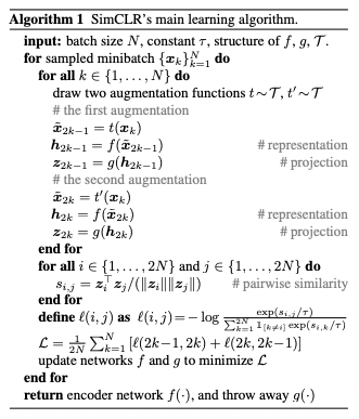
SimCLR learns representations by maximizing agreement between differently augmented views of the same data example via a contrastive loss in the latent space. The framework is composed of:
- A stochastic data augmentation module: Random crop, gaussian blur, color distortion
- A neural network base encoder f(•): ResNet
- A small neural network projection head g(•): MLP with $\bold{z_i}=g(\bold{h_i})=W^{(2)}\sigma(W^{(1)}\bold{h_i})$, while $\sigma$is ReLU non-linearity
- A contrastive loss function
Randomly sample a minibatch of N samples and define the contrastive prediction task. 2N augmented data points and 2(N-1) negative examples is generated. Let sim(u,v) as cosine similarity between u and v. Then the loss function for positive examples can be defined as
\[l_{i,j}=-\log\frac{\exp(sim(z_i,z_j)/\tau)}{\sum_{k=1}^{2N}\mathcal{1_{[k\neq\,i]}}\exp(\sim(z_i,z_j)/\tau)}\]and it calculate both (i, j) and (j, i) for all positive pairs.

Above summarizes the algorithm.
2.2. Training with Large Batch Size
Without training with a memory bank, researchers varied the training batch size N from 256 to 8192. Since the batch size is large, standard SGD / Momentum with linear learning rate scaling might not be stable, they used the LARS optimizer.
Global BN
Since in distributed training with data parallelism, the BN mean and variances tends to be aggregated locally, there is a problem with exploiting the local information and failing to learn representation. Therefore researchers aggregate BN mean and variance over all devices during the training by shuffling data examples or replacing BN with layer norm.
2.3. Evaluation Protocol
Dataset and Metrics
Unsupervised pre-training is done using the ImageNet ILSVRC-2012 dataset, and additional pre-training used CIFAR-10. To evaluate the representation, linear evaluation protocol is used, which uses frozen base network and training a linear classifier on the top of that.
Default setting
For data augmentation, random crop and resize, color distortions, gaussian blur is used. ResBet-50 is used for the base encoder, and 2-layer MLP was used as a projection head for the representation to projected into 128-dim latent space. For the loss, NT-Xent optimized with LARS with learning rate or 4.8 and weight decay of 10^-6 is used. Learning rate with the cosine decay schedule is used.
3. Data Augmentation for Contrastive Representation Learning
Data augmentation defines predictive tasks
Unlike many existing approaches approaches contrastive prediction tasks by changing the architecture, researchers tried to solve this problem with data augmentation by simple random cropping.
3.1. Composition of data augmentation operations is crucial for learning good representations
To know the impact of data augmentation, they investigated the performance of the framework by applying the augmentations individually or in pairs, always applying crop and resize, since they used the ImageNet contains different sizes. In result, single augmentation was not enough to learn good representations. Otherwise, composing augmentations, the contrastive prediction task became harder but the quality of the representation became much better. One composition of random cropping and random color distortion was outstanding, so they assumed that it was critical to compose them in order to learn generalizable features.
3.2. Contrastive learning needs stronger data augmentation than supervised learning
Stronger color augmentation seemed to substantially improves the linear evaluation of the learned unsupervised models. Compared to the supervised case which performance was not increased or hurts the performance, unsupervised case seemed to be benefitted from stronger color augmentation.
4. Architectures for Encoder and Head
4.1. Unsupervised contrastive learning benefits(more) from bigger models
Increasing depth and width both improve performance, and also decreased the gap between the linear classifiers that trained on the unsupervised model and supervised model. So, they assumed that unsupervised model benefits more than a supervised case from bigger model size.
4.2. A nonlinear projection head improves the representation quality of the layer before it
Comparing three architectures for head: identity mapping, linear projection and nonlinear projection with additional hidden layer and ReLU activation, nonlinear projection was better than linear projection by +3%. They conjecture that the representation before the nonlinear projection is important because of the loss of information induced by the contrastive loss. Since the z=g(h) is invariant to data transformation, so it could lack some information for downstream tasks. The nonlinearity can handle this problem a bit and that information remains to h. To test this idea, comparing h and g(h) as using them to learn to predict the transformation applied to the data, and the result said that h contains much more information than g(h).
5. Loss Functions and Batch Size
5.1. Normalized cross entropy loss with adjustable temperature works better than alternatives

Comparing NT-Xent with other contrastive loss functions, L2 normalization along with temperature effectively weights different examples, and set with appropriate temperature, the model could learn from hard negatives. Also, unlike Xent, other objective functions do not weigh negatives by their relative hardness. To compare them, researchers used the same L2 normalization for all loss functions, and tuned the hyperparameters for the best performance. In result, NT-Xent loss was best out of the loss functions. Without normalization or proper temperature scaling, the performance was significantly worse. L2 normalization was needed for better representation but contrastive task accuracy went low when applied.
5.2. Contrastive learning benefits (more) from larger batch sizes and longer training
With small training epochs, the larger batch size had a significant advantage over the smaller ones. In compare with the supervised case, larger batch sizes provided more negative examples and facilitating convergence.
6. Comparison with State-of-the-art
Linear evaluation

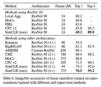
Compared to the supervised case, the model could match or outperform by the ImageNet accuracy.
Semi-supervised learning
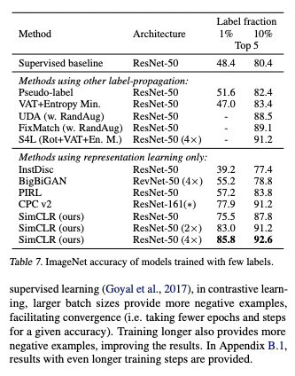
Sampling 1% or 10% of the labeled ILSVRC-12 training datasets, and fine-tuning the while base network on the labeled data without regularization, compared the result against the recent methods, and it outperformed compared to the supervised case. Fine-tuning model pre-trained on full ImageNet was better than training from the scratch.

Transfer learning

Using 12 natural image datasets, researchers evaluated the transfer learning performance of the model. In the fine-tuned cases, the model outperformed the baseline of the supervised case.


댓글남기기